6. 결정 트리
- 분류와 회귀, 다중 출력까지 가능한 다목적 머신러닝 알고리즘
- 복잡한 데이터셋도 학습 가능 (랜덤포레스트의 기본 구성 요소)
6-1 결정 트리 학습과 시각화
- Iris 데이터셋을 결정 트리 알고리즘에 피팅해본 예
from sklearn.datasets import load_iris
from sklearn.tree import DecisionTreeClassifier

iris = load_iris(as_frame=True)
X_iris = iris.data[["petal length (cm)", "petal width (cm)"]].values
y_iris = iris.target

tree_clf = DecisionTreeClassifier(max_depth=2, random_state=42)
tree_clf.fit(X_iris, y_iris)
- 결정 트리 시각화
from sklearn.tree import export_graphviz

export_graphviz(
        tree_clf,
        out_file=str(IMAGES_PATH / "iris_tree.dot"),  # 경로가 책과 다릅니다.
        feature_names=["petal length (cm)", "petal width (cm)"],
        class_names=iris.target_names,
        rounded=True,
        filled=True
    )
- graphviz : 오픈소스 그래프 시각화 소프트웨어 패키지

6-2 예측
1) 루트 노드에서 시작
2) 조건을 검사 : 검사 결과에 따라 어느 쪽 자식 노드로 이동할 지 결정
3) 리프 노드에 도달하면 멈춤
samples : 얼마나 많은 훈련 샘플이 적용되었는지 헤아린 것
value : 각 클래스에 얼마나 많은 훈련 샘플이 있는지 표시한 것
gini : 노드의 지니 불순도
* 지니 불순도: 노드에 샘플이 모두 같은 클래스면 0인 값
- 이진 트리의 결정 경계 : 수직인 선들로 데이터를 분할
* max_depth = 2일 때의 결정 경계, max_depth = 3으로 바꾸면 한번 더 데이터를 분할함
* 모델 해석
화이트박스: 직관적이고 결정 방식을 이해하기 쉬운 모델 > 결정 트리가 여기에 해당
블랙박스 : 성능이 뛰어나고 예측을 만드는 연산 과정을 쉽게 확인할 수 있음, 그러나 왜 그런 예측을 만드는 지 설명하기 어려움
> 랜덤 포레스트, 뉴럴 네트워크
6-3 클래스 확률 추정
- 결정 트리는 한 샘플이 특정 클래스에 속할 확률을 추정할 수 있음
- 주어진 샘플의 리프노드를 찾기 위해 트리를 탐색하고 그 노드에 있는 클래스 k의 훈련 샘플의 비율을 반환함
tree_clf.predict_proba([[5, 1.5]]).round(3)
array([[0. , 0.907, 0.093]])tree_clf.predict([[5, 1.5]])
>> 1개의 클래스 예측이 출력
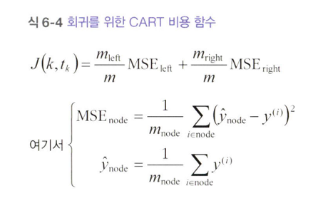
6-4 CART 훈련 알고리즘
- 사이킷런은 결정 트리를 훈련시키기 위해 CART 알고리즘을 사용함
- 훈련 세트를 하나의 특성 k의 임곗값 tk를 사용해 두 개의 서브셋으로 나눔
- k와 t_k를 고르는 방법: 가장 순수한 서브셋으로 나눌 수 있도록 하는 (k, t_k) 쌍을 알고리즘으로 찾음
* 알고리즘이 최소화해야 하는 Cost Function
- 이 과정을 반복해 불순도를 줄여 나감
6-5 계산 복잡도
- 결정 트리는 거의 균형을 이루고 있으므로 탐색에 대략 O(log_2(M))개의 노드를 거침
- 특성값 하나를 확인하기 위한 시간 복잡도가 그 정도
- 모든 샘플의 모든 특성 비교 시 : O(n*mlog_2(m))
6-6 지니 불순도 / 엔트로피
- criterion 매개변수를 'entropy' 로 지정하면 됨
- 엔트로피: 불순도를 측정하는 또 다른 지표

- 지니 불순도가 엔트로피에 비해 좀 더 계산이 빠름
6-7 규제 매개변수
- 결정 트리: 훈련되기 전에 파라미터 수가 결정되지 않음 > 비파라미터 모
- 따라서 트리가 훈련 데이터에 아주 가깝게 맞추려고 해서 오비피팅이 쉬움
* DecisionTreeClassifier의 형태를 제한하는 하이퍼파라미터들
- max_features: 각 노드에서 분할에 사용할 특성의 최대 수
- max_leaf_nodes: 리프 노드의 최대 수
- min_samples_split: 분할되기 위해 노드가 가져야 하는 최소 샘플 수
- min_samples_leaf: 리프 노드가 생성되기 위해 가지고 있어야 할 최소 샘플 수
- min_weight_fraction_leaf: min_samples_leaf와 같지만 가중치가 부여된 전체 샘플 수에서의 비율
* min으로 시작하는 매개변수를 증가시키거나 max로 시작하는 매개변수를 감소시키면 모데레 대한 규제가 커짐
from sklearn.datasets import make_moons

X_moons, y_moons = make_moons(n_samples=150, noise=0.2, random_state=42)

tree_clf1 = DecisionTreeClassifier(random_state=42)
tree_clf2 = DecisionTreeClassifier(min_samples_leaf=5, random_state=42)
tree_clf1.fit(X_moons, y_moons)
tree_clf2.fit(X_moons, y_moons)
# 추가 코드 - 이 셀은 그림 6-3을 생성하고 저장합니다.
def plot_decision_boundary(clf, X, y, axes, cmap):
x1, x2 = np.meshgrid(np.linspace(axes[0], axes[1], 100),
np.linspace(axes[2], axes[3], 100))
X_new = np.c_[x1.ravel(), x2.ravel()]
y_pred = clf.predict(X_new).reshape(x1.shape)
plt.contourf(x1, x2, y_pred, alpha=0.3, cmap=cmap)
plt.contour(x1, x2, y_pred, cmap="Greys", alpha=0.8)
colors = {"Wistia": ["#78785c", "#c47b27"], "Pastel1": ["red", "blue"]}
markers = ("o", "^")
for idx in (0, 1):
plt.plot(X[:, 0][y == idx], X[:, 1][y == idx],
color=colors[cmap][idx], marker=markers[idx], linestyle="none")
plt.axis(axes)
plt.xlabel(r"$x_1$")
plt.ylabel(r"$x_2$", rotation=0)
fig, axes = plt.subplots(ncols=2, figsize=(10, 4), sharey=True)
plt.sca(axes[0])
plot_decision_boundary(tree_clf1, X_moons, y_moons,
axes=[-1.5, 2.4, -1, 1.5], cmap="Wistia")
plt.title("No restrictions")
plt.sca(axes[1])
plot_decision_boundary(tree_clf2, X_moons, y_moons,
axes=[-1.5, 2.4, -1, 1.5], cmap="Wistia")
plt.title(f"min_samples_leaf = {tree_clf2.min_samples_leaf}")
plt.ylabel("")
save_fig("min_samples_leaf_plot")
plt.show()

from sklearn.tree import DecisionTreeRegressor

np.random.seed(42)
X_quad = np.random.rand(200, 1) - 0.5  # 간단한 랜덤한 입력 특성
y_quad = X_quad ** 2 + 0.025 * np.random.randn(200, 1)

tree_reg = DecisionTreeRegressor(max_depth=2, random_state=42)
tree_reg.fit(X_quad, y_quad)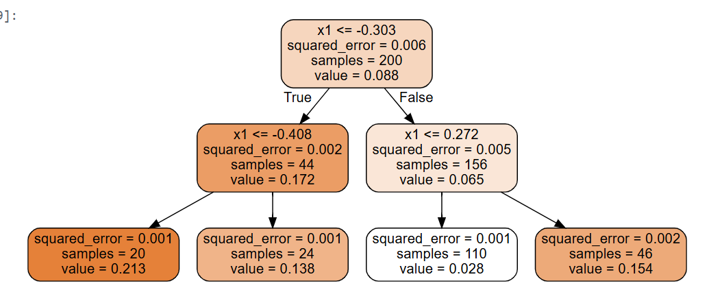
- 형태: 유사
- 차이: 각 노드에서 클래스를 예측하려고 하는 대신 어떤 값을 예측
* 회귀를 위한 CART 알고리즘 Cost Function
6-9 축 방향에 대한 민감성
- 결정 트리는 결정 경계가 항상 계단 모양 : 수직 방향의 분할만 가능
- 해결: 데이터의 스케일을 조정하고 PCA를 사용하여 데이터를 회전시키는 작은 파이프라인을 만든 다음 이 데이터에서 DecisionTreeClassifier를 훈련
from sklearn.decomposition import PCA
from sklearn.pipeline import make_pipeline
from sklearn.preprocessing import StandardScaler

pca_pipeline = make_pipeline(StandardScaler(), PCA())
X_iris_rotated = pca_pipeline.fit_transform(X_iris)
tree_clf_pca = DecisionTreeClassifier(max_depth=2, random_state=42)
tree_clf_pca.fit(X_iris_rotated, y_iris)
6- 10 결정 트리의 분산 문제
- 사이킷런에서 사용하는 CART 학습 알고리즘은 확률적
- 동일한 데이터에 대해 동일한 모델을 학습하더라도 매번 매우 다른 모델이 생성될 수 있다는 의미
7. 앙상블 학습과 랜덤 포레스트
- 비슷한 일련의 예측기로부터 예측을 수집하면 가장 좋은 분류기 하나보다 더 나은 예측을 만들 수 있다!
7-1 투표 기반 분류기
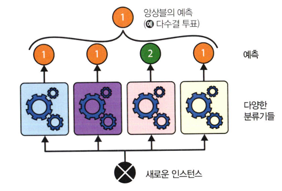
- 직접 투표 분류기: 각 분류기의 예측을 집계해 가장 많이 나온 클래스로 결정하는 것
- 약한 학습기: 랜덤 추측보다 조금 나은 성능을 보이는 분류기
- 강한 학습기: 높은 정확도를 내는 분류
- 각 분류기가 약한 학습기일지라도 다양하고 많다면 앙상블은 강한 학습기가 됨
* 이유: 큰 수의 법칙 때문!

: 51% 정확도의 분류기 1000개 모으면 75% 정확도를 기대할 수 있음
* VotingClassifier
from sklearn.datasets import make_moons
from sklearn.ensemble import RandomForestClassifier, VotingClassifier
from sklearn.linear_model import LogisticRegression
from sklearn.model_selection import train_test_split
from sklearn.svm import SVC

X, y = make_moons(n_samples=500, noise=0.30, random_state=42)
X_train, X_test, y_train, y_test = train_test_split(X, y, random_state=42)

voting_clf = VotingClassifier(
    estimators=[
        ('lr', LogisticRegression(random_state=42)),
        ('rf', RandomForestClassifier(random_state=42)),
        ('svc', SVC(random_state=42))
    ]
)
voting_clf.fit(X_train, y_train)
> 투표 기반이 개별 분류기보다 높은 성능
간접 투표: 개별 분류기의 예측을 평균 내어 가장 높은 클래스를 예측하는 것
7-2 배깅과 페이스팅
배깅: 훈련 세트에서 중복을 허용하여 샘플링하는 방식
페이스팅: 중복을 허용하지 않고 샘플링하는 방식

- 분류: 통계적 최빈값을 예측을 결과로
-회귀: 예측값들의 평균
- 다른 CPU 코어나 서버에서 병렬로 학습 가능
from sklearn.ensemble import BaggingClassifier
from sklearn.tree import DecisionTreeClassifier

bag_clf = BaggingClassifier(DecisionTreeClassifier(), n_estimators=500,
                            max_samples=100, n_jobs=-1, random_state=42)
bag_clf.fit(X_train, y_train)
# 추가 코드 - 이 셀은 그림 7-5를 생성하고 저장합니다.
def plot_decision_boundary(clf, X, y, alpha=1.0):
axes=[-1.5, 2.4, -1, 1.5]
x1, x2 = np.meshgrid(np.linspace(axes[0], axes[1], 100),
np.linspace(axes[2], axes[3], 100))
X_new = np.c_[x1.ravel(), x2.ravel()]
y_pred = clf.predict(X_new).reshape(x1.shape)
plt.contourf(x1, x2, y_pred, alpha=0.3 * alpha, cmap='Wistia')
plt.contour(x1, x2, y_pred, cmap="Greys", alpha=0.8 * alpha)
colors = ["#78785c", "#c47b27"]
markers = ("o", "^")
for idx in (0, 1):
plt.plot(X[:, 0][y == idx], X[:, 1][y == idx],
color=colors[idx], marker=markers[idx], linestyle="none")
plt.axis(axes)
plt.xlabel(r"$x_1$")
plt.ylabel(r"$x_2$", rotation=0)
tree_clf = DecisionTreeClassifier(random_state=42)
tree_clf.fit(X_train, y_train)
fig, axes = plt.subplots(ncols=2, figsize=(10, 4), sharey=True)
plt.sca(axes[0])
plot_decision_boundary(tree_clf, X_train, y_train)
plt.title("결정 트리")
plt.sca(axes[1])
plot_decision_boundary(bag_clf, X_train, y_train)
plt.title("배깅을 사용한 결정 트리")
plt.ylabel("")
save_fig("decision_tree_without_and_with_bagging_plot")
plt.show()
- 결정 트리와 배깅을 사용한 결정 트리의 비교
* OOB 평가
- BaggingClassifier는 기본값으로 중복을 허용하여(bootstrap=True) 훈련 세트의 크기만큼인 m개 샘플을 선택함
: 따라서 평균적으로 각 예측기에 훈련 샘플의 63% 정도만 샘플링에 포함
>> 남은 37%의 샘플을 평가에 사용 가능!
bag_clf = BaggingClassifier(DecisionTreeClassifier(), n_estimators=500,
                            oob_score=True, n_jobs=-1, random_state=42)
bag_clf.fit(X_train, y_train)
bag_clf.oob_score_
0.896bag_clf.oob_decision_function_[:3] # probas for the first 3 instances
array([[0.32352941, 0.67647059],
       [0.3375    , 0.6625    ],
       [1.        , 0.        ]])
7-4 랜덤 포레스트
랜덤 포레스트: 배깅 또는 페이스팅 방법을 적용한 결정 트리 앙상블
엑스트라 트리: 트리를 더욱 랜덤하게 만들기 위해, 후보 특성을 사용해 랜덤으로 분할한 후 그중 최상의 분할을 선택한 것
> 극단적으로 랜덤하면 익스트림 랜덤 트리
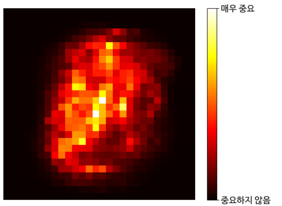
특성 중요도: 어떤 특성을 사용한 노드가 평균적으로 불순도를 얼마나 감소시키는지 확인하여 특성 중요도 측정
from sklearn.datasets import fetch_openml

# 사이킷런 1.4버전에서 parser 매개변수 기본값이 'liac-arff'에서 'auto'로 바뀌었습니다.
# 이전 버전에서도 동일한 결과를 내도록 명시적으로 'auto'로 지정합니다.
X_mnist, y_mnist = fetch_openml('mnist_784', return_X_y=True,
                                as_frame=False, parser='auto')

rnd_clf = RandomForestClassifier(n_estimators=100, random_state=42)
rnd_clf.fit(X_mnist, y_mnist)

heatmap_image = rnd_clf.feature_importances_.reshape(28, 28)
plt.imshow(heatmap_image, cmap="hot")
cbar = plt.colorbar(ticks=[rnd_clf.feature_importances_.min(),
                           rnd_clf.feature_importances_.max()])
cbar.ax.set_yticklabels(['중요하지 않음', '매우 중요'], fontsize=14)
plt.axis("off")
save_fig("mnist_feature_importance_plot")
plt.show()
7-5 부스팅
: 앞의 모델을 보완해 나가면서 일련의 예측기를 학습하는 것
- AdaBoost
m = len(X_train)

fig, axes = plt.subplots(ncols=2, figsize=(10, 4), sharey=True)
for subplot, learning_rate in ((0, 1), (1, 0.5)):
    sample_weights = np.ones(m) / m
    plt.sca(axes[subplot])
    for i in range(5):
        svm_clf = SVC(C=0.2, gamma=0.6, random_state=42)
        svm_clf.fit(X_train, y_train, sample_weight=sample_weights * m)
        y_pred = svm_clf.predict(X_train)

        error_weights = sample_weights[y_pred != y_train].sum()
        r = error_weights / sample_weights.sum()  # equation 7-1
        alpha = learning_rate * np.log((1 - r) / r)  # equation 7-2
        sample_weights[y_pred != y_train] *= np.exp(alpha)  # equation 7-3
        sample_weights /= sample_weights.sum()  # normalization step

        plot_decision_boundary(svm_clf, X_train, y_train, alpha=0.4)
        plt.title(f"learning_rate = {learning_rate}")
    if subplot == 0:
        plt.text(-0.75, -0.95, "1", fontsize=16)
        plt.text(-1.05, -0.95, "2", fontsize=16)
        plt.text(1.0, -0.95, "3", fontsize=16)
        plt.text(-1.45, -0.5, "4", fontsize=16)
        plt.text(1.36,  -0.95, "5", fontsize=16)
    else:
        plt.ylabel("")

save_fig("boosting_plot")
plt.show()

from sklearn.ensemble import AdaBoostClassifier

ada_clf = AdaBoostClassifier(
    DecisionTreeClassifier(max_depth=1), n_estimators=30,
    learning_rate=0.5, random_state=42)
ada_clf.fit(X_train, y_train)
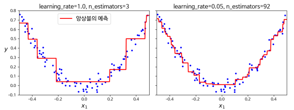
- 그레이디언트 부스팅
def plot_predictions(regressors, X, y, axes, style,
                     label=None, data_style="b.", data_label=None):
    x1 = np.linspace(axes[0], axes[1], 500)
    y_pred = sum(regressor.predict(x1.reshape(-1, 1))
                 for regressor in regressors)
    plt.plot(X[:, 0], y, data_style, label=data_label)
    plt.plot(x1, y_pred, style, linewidth=2, label=label)
    if label or data_label:
        plt.legend(loc="upper center")
    plt.axis(axes)

plt.figure(figsize=(11, 11))

plt.subplot(3, 2, 1)
plot_predictions([tree_reg1], X, y, axes=[-0.5, 0.5, -0.2, 0.8], style="g-",
                 label="$h_1(x_1)$", data_label="훈련 세트")
plt.ylabel("$y$  ", rotation=0)
plt.title("잔여 오차와 트리의 예측")

plt.subplot(3, 2, 2)
plot_predictions([tree_reg1], X, y, axes=[-0.5, 0.5, -0.2, 0.8], style="r-",
                 label="$h(x_1) = h_1(x_1)$", data_label="훈련 세트")
plt.title("앙상블의 예측")

plt.subplot(3, 2, 3)
plot_predictions([tree_reg2], X, y2, axes=[-0.5, 0.5, -0.4, 0.6], style="g-",
                 label="$h_2(x_1)$", data_style="k+",
                 data_label="잔여 오차: $y - h_1(x_1)$")
plt.ylabel("$y$  ", rotation=0)

plt.subplot(3, 2, 4)
plot_predictions([tree_reg1, tree_reg2], X, y, axes=[-0.5, 0.5, -0.2, 0.8],
                  style="r-", label="$h(x_1) = h_1(x_1) + h_2(x_1)$")

plt.subplot(3, 2, 5)
plot_predictions([tree_reg3], X, y3, axes=[-0.5, 0.5, -0.4, 0.6], style="g-",
                 label="$h_3(x_1)$", data_style="k+",
                 data_label="잔여 오차: $y - h_1(x_1) - h_2(x_1)$")
plt.xlabel("$x_1$")
plt.ylabel("$y$  ", rotation=0)

plt.subplot(3, 2, 6)
plot_predictions([tree_reg1, tree_reg2, tree_reg3], X, y,
                 axes=[-0.5, 0.5, -0.2, 0.8], style="r-",
                 label="$h(x_1) = h_1(x_1) + h_2(x_1) + h_3(x_1)$")
plt.xlabel("$x_1$")

save_fig("gradient_boosting_plot")
plt.show()
from sklearn.ensemble import GradientBoostingRegressor
gbrt = GradientBoostingRegressor(max_depth=2, n_estimators=3,
learning_rate=1.0, random_state=42)
gbrt.fit(X, y)